Scraping

For scraping, I found this wonderful walkthrough by Ashley Kelnhofer, with code by Justin Gale, that uses Google Apps Script to populate a Google Sheet with calendar events.

I needed a guest record, so I hacked on a for loop, to return the event’s guest list, my tweaks are in a GIST here.

Importing

library(googlesheets) is a great package by Jenny Bryan and it makes getting data out of your Google Sheets and into data frames simple. I like Google Sheets with R because it gives you an access point to get data from other Google Apps and makes sharing data easy without requiring Git skills.

library(googlesheets4) # gs_verb()

gs4_auth("nathan.day@hemoshear.com")
# oAuth2, so browser confirmation req'd

events <- gs4_find() %>%
  select(name, id) %>%
  filter(grepl("Calendar", name)) %>%
  deframe() %>% 
  map_df(read_sheet, .id = "cal")

names(events) %<>% tolower() %>% gsub(" ", "_", .)
names(events)

Remember guest_email is the field I hacked together in Google Apps Script with my_array.join() and it looks like this, “myname@mail.com,yourname@mail.com”

Exploring

A look at the duration distribution.

ggplot(events, aes(calculated_duration)) +
  geom_histogram(bins = 10) +
  labs(y = "# Meetings", x = "Meeting length (hours)")

Tells us most meetings are about an hour or less and that’s good to see that we are keeping things short. But we did have some meeting marathons, that were over 4 hours long.

I was also currious if there was a difference between the two confernce rooms.

events %>%
  filter(grepl("Conference", cal)) %>%
  ggplot(aes(calculated_duration)) +
    geom_histogram(bins = 10) +
    facet_wrap(~cal) +
    labs(y = "# Meetings", x = "Meeting length (hours)")

I see a lot more meetings used the big conference room, which might mean most of our meetings have a lot of attendees.

To answer that we need to extract the individual emails that are currently packed as csvs in guest_email.

events %<>% separate_rows(guest_email, sep = ",")

Dang, tidyr::separate_rows() is a great function and why I decided to to transport the data in this format. It is a useful pattern for bring array data into R from other languages.

It turns out some of the “attendees” on the guest list are actually WebX robots, so I dropped them. There were also NA values, becasue some meetings didn’t have guest-lists, so those had to go too.

events %<>% filter(!grepl("google", guest_email), !is.na(guest_email))

Now to see if the meetings in the bigger room do actually have more people?

events %>%
  filter(grepl("Conference", cal)) %>%
  group_by(cal, event_start) %>%
  summarise(people = n()) %>%
  ggplot(aes(people)) +
    geom_histogram(bins = 5) +
    facet_wrap(~cal) +
    labs(x = "Attendees", y = "# Meetings")

Sure enough the meetings in the big conference room do tend to be larger. But its good to see most of our meeting have less than 10 people.

Note: that these guest lists included people calling in for meetings too. Just in case anyone is thinking we are breaking fire code by cramming 30+ people into a room for 14

I think meetings work best with 4-5 peole, because at that size everyone is contributing to the discussion. Smaller groups also makes hearing quieter voices easier. I think people would be amazed at a what they get done with smaller meetings and larger email recaps.

Finally let’s look at individual employees and see how many hours each spent in meetings for August. For reference August had 23 work-day for a total of 184 work-hours.

This is what the company org chart looks like.

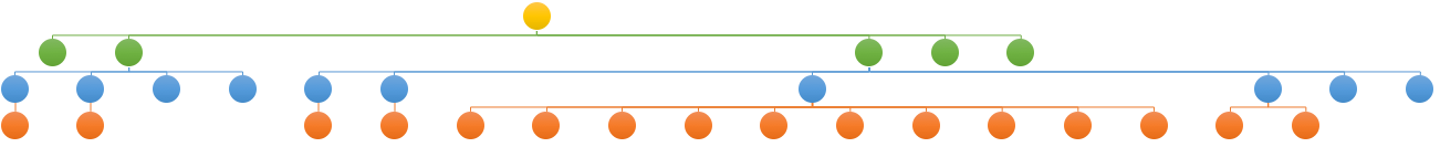
org-chart

And this bar chart shows each individual’s cumulative meeting hours for August.

cust_colors <- c("#fcd432", "#33b716", "#0688ce", "#e85906", "#A9A9A9") %>%
  set_names(c("ceo", "executive", "director", "staff", "external"))

events %>%
  group_by(guest_email, job_title) %>%
  filter(n() > 2) %>% 
  summarise(total_time = sum(calculated_duration)) %>% 
  ungroup() %>%
  mutate(guest_email = fct_reorder(guest_email, total_time),
         job_title = factor(job_title, names(cust_colors))) %>%
  ggplot(aes(guest_email, total_time, label = guest_email, fill = job_title)) +
    geom_col() +
    scale_y_continuous(breaks = seq(10, 80, 10)) +
    scale_fill_manual(values = cust_colors) +
    labs(y = "Hours in meetings", x = "Employee") +
    theme(axis.text.x = element_blank())

We can see 6 employees that spent over one full work week (40 hours) in meetings. One of the external consultants also logged 20 hours, which seemed like a lot for a part-time consulting position The relativly low hours for our CEO was suprising to see.