Introduction

For over a year now I have wanted to learn how to use R’s non-standard evaluation and dispite reading the developer rules and Hadley’s Adv-R section multiple times, I never really made any progress understanding it. Then I saw Edwin Thoen’s NSE/tidyveal post and it kinda (key word) started to click. Edwin’s follow up about common use cases was the turning point for me and I gradually started using things like !! and writing functions with my favorite tidyverse tools.

I still don’t feel like I have a great handle on NSE, but when I saw [@coolbutuseless's tweet](https://twitter.com/coolbutuseless/status/969853912990720005) yesteday about tidyverse replacements for the deprecated group_by %>% dplyr::do() I decided to try and build a tidyverse incarnation of split(), that captured bar column names to split on, similar to how dplyr::select() works. The way I do split-apply-combine now is with data %>% split(list(.$col1, .$col2), drop = TRUE) %>% map_df() and I use this all the time pretty much in every script. I’ve always just thought of the .$ syntax as neccesary overhead to use this code template, but it turns out my tidyverse incarnation runs faster than base::split()!!!

In additional to the resources above, I finally watched Lionel Henry’s Tidy Eval presentation this morning and I couldn’t have written this function without it. If you are struggling to understand the wacky world of quosure, like me, he does a great walk-through. This method is an adpation of the cement() example function from his presentation.

My tidy try: split_()

library(rlang)
library(tidyverse)

library(rlang)
library(tidyverse)

split_ <- function(data, ..., .drop = TRUE) {
    vars <- ensyms(...)
    vars <- map(vars, function(x) eval_tidy(x, data))
    split(data, vars, drop = .drop)
}

I don’t think I’ve spent this long writing three lines of code since I first learned about ggplot(). Getting this right took me a long time, because NSE is confusing and dealing with a list of quosures was opaque to me, until I watched Lionel’s walk through.

The idea of using the ... is to capture all of the unnamed argument passed into split_() and it is how other tidyverse staples like dplyr::select() work, so I could template my function off of those. This allows me to pass any number of column names in, but it doesn’t allow the tricks of dplyr::vars() like negation indexing (-cyl) or index ranges (cyl:vs), so that’s something to shoot for.

rlang::ensyms() is the plural form of ensym(), which allows multiple values to be captured. Both of these functions are similar to rlang::enexpr(), which captures raw expressions and saves them for evaluation later. The only diffence with the ensym varieties is that they check if the captured expression is either a string or symbol and then convert any strings to symbols. This gives us some flexibilty for passing in arguments either as quoted or bare column names, even though we likely want to always use bare ones.

Then purrr::map() is iterating over each symbol in our list using tidy_eval to evaluate each on within the environment of data. Since data is a data.frame() that means we are getting back columns, which we will just keep in the list and pass to base::split() as the f argument. This function will fail if a name passed in ... can’t be found in names(data), but that’s consistant with other functions.

summarise(mtcars, avg = mean(Sepal.Length))

## Error: Problem with `summarise()` input `avg`.
## x object 'Sepal.Length' not found
## ℹ Input `avg` is `mean(Sepal.Length)`.

split_(mtcars, Sepal.Length)

## Error in eval_tidy(x, data): object 'Sepal.Length' not found

I set the default to drop = TRUE, because thats how I use split now, but kept the option to pass through via the .drop argument. I could expand with split_()’s other arguments. but this is about the NSE exploration.

I am most definatly a tidy eval novice and the reason I wrote this up was so I would have to articulate what I know (or think I know) about how it does it’s dark magic. So I hope this helps, but I highly reccommend getting a more expert take on this topic from the links above.

Tests!!!

# adapted from the last example on ?purrr::map
mtcars %>%
  split_(cyl, vs) %>%
  map_df(~ broom::tidy(lm(mpg ~ wt, data = .)),
         .id = "cyl")

## # A tibble: 9 x 6
##   cyl   term        estimate std.error statistic      p.value
##   <chr> <chr>          <dbl>     <dbl>     <dbl>        <dbl>
## 1 4.0   (Intercept)   26       NaN       NaN     NaN         
## 2 6.0   (Intercept)   22.2      16.1       1.38    0.399     
## 3 6.0   wt            -0.594     5.83     -0.102   0.935     
## 4 8.0   (Intercept)   23.9       3.01      7.94    0.00000405
## 5 8.0   wt            -2.19      0.739    -2.97    0.0118    
## 6 4.1   (Intercept)   39.9       4.61      8.66    0.0000247 
## 7 4.1   wt            -5.72      1.95     -2.94    0.0187    
## 8 6.1   (Intercept)   63.6      11.9       5.36    0.0330    
## 9 6.1   wt           -13.1       3.50     -3.75    0.0642

I wonder if anyone has ever made a straight 8 engine…

cleave_by()

When I went back to grab the link for the original tweet that got be started on this, @coolbutuseless (OP) had already built another implemention of the same idea they called cleave_by()!!! Here is their version, which looks like it might become part of tidyr:

# https://coolbutuseless.bitbucket.io/2018/03/04/cleave_by-a-tidyverse-style-split/

cleave_by <- function(df, ...) {
    stopifnot(inherits(df, "data.frame"))
    
    # use tidyeval to get the names ready for dplyr
    grouping <- quos(...)
    
    # Calculate a single number to represent each group
    group_index <- df %>%
        group_by(!!!grouping) %>%
        group_indices()
    
    # do the split by this single group_index variable and return it
    split(df, group_index)
}

And it looks like They also ran two series of benchmarks to compare runtimes for their cleave_by() and base::split(). So I figured I would throw split_() into the ring and see how it did.

I want to point out that @coolbutuseless’s version has some nice features over the base::split() which they discuss in their blogpost and it’s a safer than my original attemp. Since these safety improvments, like class checking are extra function calls, I’m going to update my version, to match their behavior of class checking and NA retention.

# updated v2
split_ <- function(data, ..., .drop = TRUE) {
    stopifnot(inherits(data, "data.frame"))
    vars <- ensyms(...)
    vars <- map(vars, function(x) factor(eval_tidy(x, data), exclude = NULL))
    split(data, vars, drop = .drop)
}

Most of the code below is from [@coolbuuseless's blog post](https://coolbutuseless.bitbucket.io/) I just added the ggplot bit to approximate their plots.

set.seed(1)

create_test_df <- function(cols, rows, levels_per_var) {
    data_source <- letters[seq(levels_per_var)]
    
    create_column <- function(...) {sample(data_source, size = rows, replace = TRUE)}
    letters[seq(cols)] %>% 
        set_names(letters[seq(cols)]) %>%
        purrr::map_dfc(create_column) 
}

test_df <- create_test_df(cols=10, rows=10, levels_per_var=2)

library(microbenchmark)
bench <- microbenchmark(
    split(test_df, test_df[, c('a'                              )]),
    split(test_df, test_df[, c('a', 'b'                         )]),
    split(test_df, test_df[, c('a', 'b', 'c'                    )]),
    split(test_df, test_df[, c('a', 'b', 'c', 'd'               )]),
    split(test_df, test_df[, c('a', 'b', 'c', 'd', 'e'          )]),
    split(test_df, test_df[, c('a', 'b', 'c', 'd', 'e', 'f'     )]),
    split(test_df, test_df[, c('a', 'b', 'c', 'd', 'e', 'f', 'g')]),
    cleave_by(test_df, a),
    cleave_by(test_df, a, b),
    cleave_by(test_df, a, b, c),
    cleave_by(test_df, a, b, c, d),
    cleave_by(test_df, a, b, c, d, e),
    cleave_by(test_df, a, b, c, d, e, f),
    cleave_by(test_df, a, b, c, d, e, f, g),
    split_(test_df, a),
    split_(test_df, a, b),
    split_(test_df, a, b, c),
    split_(test_df, a, b, c, d),
    split_(test_df, a, b, c, d, e),
    split_(test_df, a, b, c, d, e, f),
    split_(test_df, a, b, c, d, e, f, g)
)

bench %>%
    mutate(func = gsub("\\(.*", "", expr)) %>%
    arrange(expr) %>%
    group_by(func) %>% 
    mutate(split_vars = rep(1:7, each = 100)) -> bench


ggplot(bench, aes(split_vars, time, color = func)) +
    stat_smooth(se = F)

## `geom_smooth()` using method = 'loess' and formula 'y ~ x'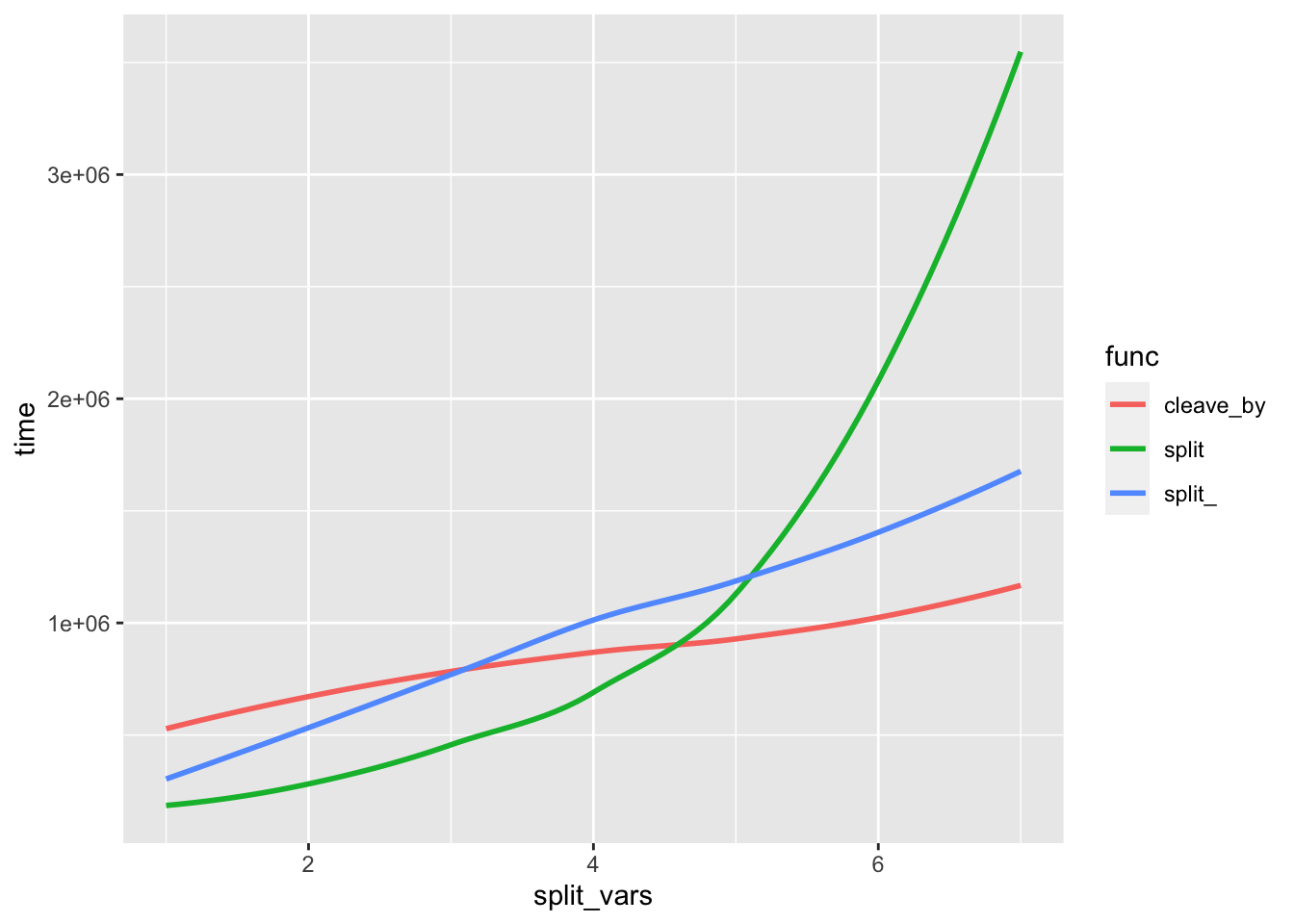

Not too shabby and I can’t tell you why my incarnation works slightly faster than the others for lower numbers of split_vars except that I did what Lionel did. I think it’s interesting how cleave_by() is noticable quicker at higher split_vars, and I need to re-read the explination for a few more times before I get it.

Here is test two, again all [@coolbutuseless](https://coolbutuseless.bitbucket.io/) plus my ggplot prep.

set.seed(2)

test_df2  <- create_test_df(cols=4, rows=40, levels_per_var= 2)
test_df3  <- create_test_df(cols=4, rows=40, levels_per_var= 3)
test_df4  <- create_test_df(cols=4, rows=40, levels_per_var= 4)
test_df5  <- create_test_df(cols=4, rows=40, levels_per_var= 5)
test_df6  <- create_test_df(cols=4, rows=40, levels_per_var= 6)  

bench2 <- microbenchmark(
    split(test_df2 , test_df2[, c('a', 'b', 'c')]),
    split(test_df3 , test_df3[, c('a', 'b', 'c')]),
    split(test_df4 , test_df4[, c('a', 'b', 'c')]),
    split(test_df5 , test_df5[, c('a', 'b', 'c')]),
    split(test_df6 , test_df6[, c('a', 'b', 'c')]),
    cleave_by(test_df2, a, b, c),
    cleave_by(test_df3, a, b, c),
    cleave_by(test_df4, a, b, c),
    cleave_by(test_df5, a, b, c),
    cleave_by(test_df6, a, b, c),
    split_(test_df2, a, b, c),
    split_(test_df3, a, b, c),
    split_(test_df4, a, b, c),
    split_(test_df5, a, b, c),
    split_(test_df6, a, b, c)
)

bench2 %>%
    mutate(func = gsub("\\(.*", "", expr)) %>%
    arrange(expr) %>%
    group_by(func) %>% 
    mutate(num_levels = rep(2:6, each = 100)) -> bench2


ggplot(bench2, aes(num_levels, time, color = func)) +
    stat_smooth(se = F)

## `geom_smooth()` using method = 'loess' and formula 'y ~ x'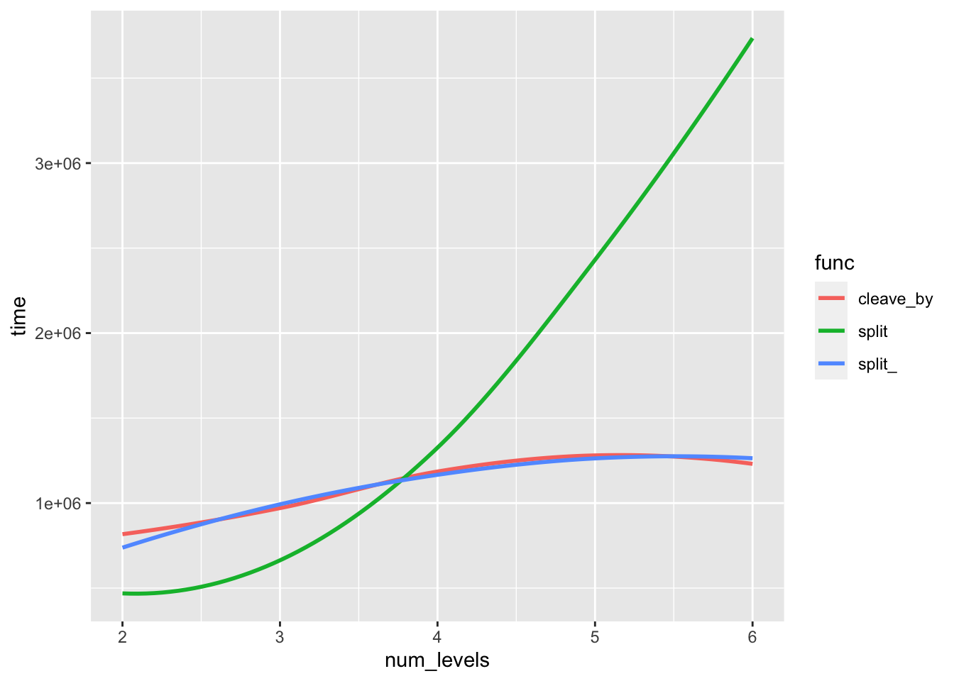

In that second test the two tidy eval versions are almost identical and only slightly worse than base::split() at the lowest number of levels.

Conclusion

I’m excited to keep exploring tidyeval and I’d like understand why the performance varies slightly. But after a year of what felt like banging my head against the wall I’m finally starting to understand how to use tidyeval. Having tangible examples like Edwin’s common cases, was a game changer for me, becasue it allowed me to really start practicing and playing with the rlang functions. Also huge thanks for the Twitter inspiration @coolbutuseless!