Intro

In my last post I spent a lot of time visualizing the drug crime data published by the Charlottesville Police Department, with library(sf). This is the peanut butter to that viz jelly, the statistical testing tools that can measure the significance of the trends we observed. And who doens’t like PB&Js?

Globals

library(geojsonio) # last two posts
library(sf) # last post
library(viridis) # last post

# library(spatstat) # new
library(spdep) # new
library(tidycensus) # new

library(magrittr) # %<>% life
library(tidyverse)

# some custom functions to make my fingers happy
theme_set(theme_grey() + theme(legend.position = "top"))
scale_fill_continuous <- function(...) { viridis::scale_fill_viridis(option = "A", ...) }

Data Input

This is block of code is aggregated from my other posts revolving around the the city’s crime data. It handles a lot of the weirdness in the original data set that needs cleaning attention. For this I’m leaving little comments as bread crumbs, if you need the whole loaf check out the earlier posts or send me an email.

# get geo-coded crime data from my GitHub
crime <- read.csv("https://raw.githubusercontent.com/NathanCDay/cville_crime/master/crime_geocode.csv")
crime %<>% filter(complete.cases(crime)) # not all raw address could be geo_coded
names(crime) %<>% tolower() # safer/easier
crime %<>% mutate(drug_flag = ifelse(grepl("drug", offense, ignore.case = TRUE),
                                     "drugs", "not_drugs")) # flag drug related crimes
crime %<>% filter(offense != "DRUG AWARENESS PRESENTATION") # drop DARE class (90's kids hands up)
crime %<>% filter(address != "600 E MARKET ST Charlottesville VA") # drop the Police Station block (fishy)

# get census data for shapes and housing data
census <- geojson_read("https://opendata.arcgis.com/datasets/e60c072dbb734454a849d21d3814cc5a_14.geojson",
                       what = "sp")
names(census) %<>% tolower()
census %<>% st_as_sf() # convert to sf object
census %<>% select(geometry, starts_with("hu"), white, black, pop = population, objectid, blockgroup) # select important columns

# filter via spatial overlay
crime %<>% st_as_sf(coords = c("lon", "lat"), crs = st_crs(census)) # project crime onto census CRS
crime %<>% mutate(objectid = st_within(crime, census) %>% as.numeric()) # returns NA for those outside
crime %<>% filter(!is.na(objectid))

Oh the things we do for reproducible scripts. Now that is out of the way we are ready to jump into testing.

Areal Stats

This type of statistics uses regions to summarize indivdual cases. Here I’m using Census blocks (again) as our region boundaries, because census data is well curated and contains a ton of meta data that we can use later on in modeling.

So the first step is to summarise the observaction in crime by shapes in census.

st_geometry(crime) <- NULL # remove sf geometry, back to basic tibble

crime %<>% group_by(objectid, drug_flag) %>% # count totals by census block
    count() %>%
    spread(drug_flag, n) %>%  # calculate fraction of drug related crime
    mutate(frac_drugs = drugs / not_drugs)

census %<>% inner_join(crime) # merge into census

Moran’s I

The first test statistic to learn for spatial data is Moran’s I. This is used to measure spatial autocorrelation, in other words are adjacent areas likely to have similar signals. The test statstic I ranges from -1 (pure dispersion) to 1 (pure clustering) with a value of 0 being random. Morans’ I is implemented in the R library(spdep) and I will focus on the function moran.mc(), which performs a Monte Carlo simulation under the hood to establish rank.

First we have to convert our sf objects into a SpatialPolygons objects, then we can use a couple other functions from library(spdep) to construct a weighted list of neigbors which is required to run moran.mc().

census_sp <- as(census, "Spatial") # convert to spatial object type

census_wnb <- spdep::poly2nb(census_sp) %>% # convert polygons to neighbor list
     spdep::nb2listw() # weight the list by 

spdep::moran.mc(census_sp$frac_drugs, census_wnb, nsim = 999) # 999+1 simulations

## 
##  Monte-Carlo simulation of Moran I
## 
## data:  census_sp$frac_drugs 
## weights: census_wnb  
## number of simulations + 1: 1000 
## 
## statistic = 0.21778, observed rank = 984, p-value = 0.016
## alternative hypothesis: greater

ggplot(census) + geom_sf(aes(fill = frac_drugs))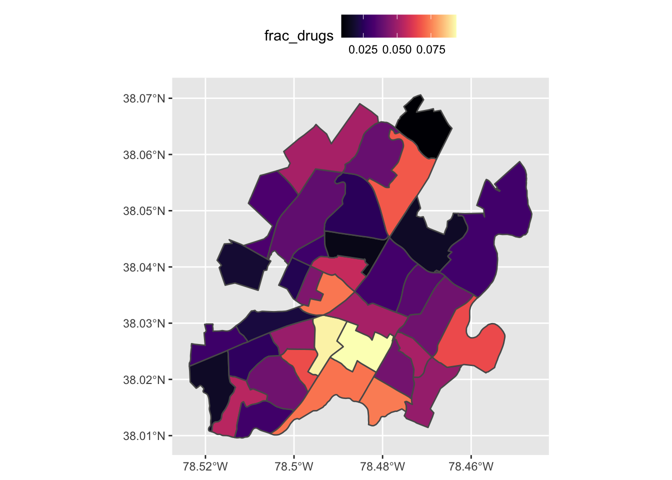

sp::spplot(census_sp, zcol = "frac_drugs") # perhaps easier/faster???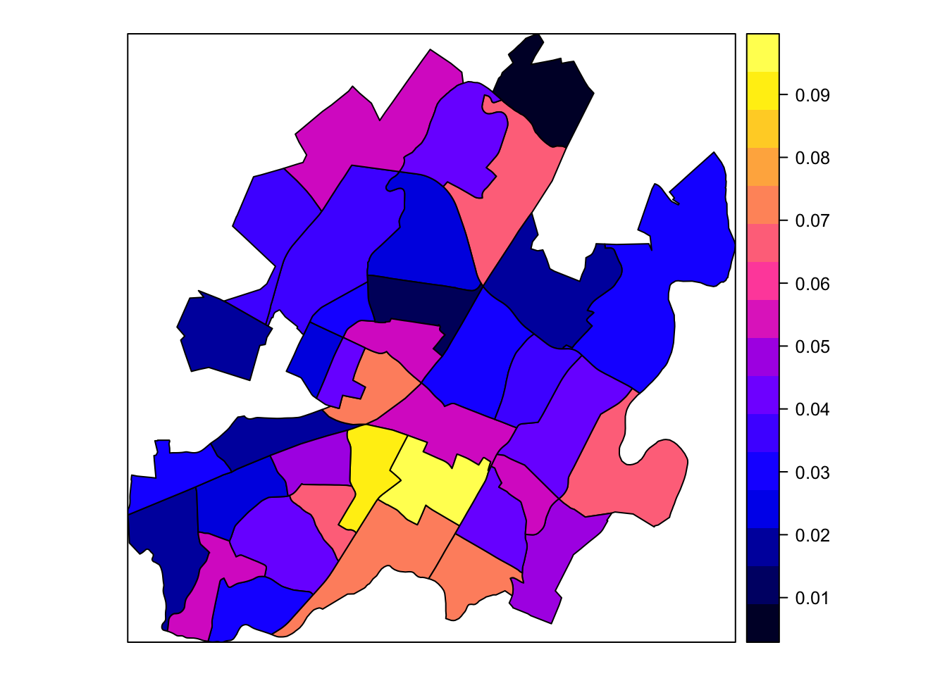

Either way you plot it, its easy to see that the SW corner of the city has a larger fraction of drug crime than either of the other three. But now we can say with a statistic greater than 0, that we are observing a clustering pattern in the fraction of drug crime. A statistic value of 0 would indicate a true random pattern and one under 0, a dispearsal pattern.

MORE DATA!!!

If we want to investigate more, we need more data. The stock census data has some housing and demographic data that might be useful, but we want more. Realistically we’d like to scan a bunch of indicators, but here we will just grab median income and age by Census block. This data is from the American Community Survey is readily available via good guy Kyle Walk and his bomb package tidycensus package. So go ahead and put those parsing pants away.

All you really have to do is register an API key here wait a couple of minutes, check your email and from there it’s all slick functions from there.

# census_api_key("your_key")

cvl <- get_acs(geography = "block group", county = "Charlottesville", state = "VA",
               variables = c("B19013_001", "B01002_001"), output = "tidy") # income & age

# the rest is cleaning...
decode <- c("income", "age") %>% set_names(c("B19013_001", "B01002_001")) # named vecs ftw
cvl$variable %<>% decode[.] # recip pipe is so nice

cvl %<>% select(GEOID, variable, estimate) %>% spread(variable, estimate) # spread to tidy

census %<>% full_join(rename(cvl, blockgroup = GEOID)) # two block have missing income values

Explore that

Great now we have a couple of extra variables to work with. But before we just blindly throw them into a model, let’s look at all of the relationships quickly via GGally::ggpairs(). Before we do that I want to build variables for the proportion of vacant homes and the population that identifies as black.

census %<>% mutate(frac_vacant = hu_vacant / (hu_occupied + hu_vacant),
                   frac_black = black / pop)

col_index <- match(c("frac_drugs", "frac_vacant", "age", "income", "frac_black"), names(census))

GGally::ggpairs(census, col_index)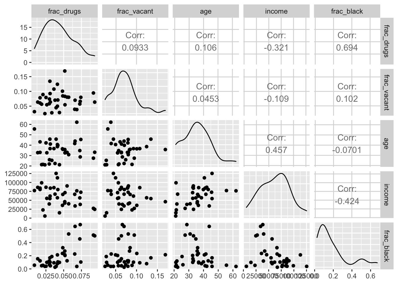

We can see that the fraction of drug crime is positively related to the fraction of the comminity that is black, the fraction of the homes that are vacant and negatively related to income. This is not suprising since America has well documented history of using drug laws to target minorities, especially black communities.

Model time

Since our respons variable is a the proportion of drug crime to total crime and is bounded by 0 and 1, we are best off using a quasi-binomial distribution. If we were using the total count of drug crimes as our response, we’d want to use a Poisson or quasipoisson distribution instead. R’s flexible glm() makes either of these scenarios simple to code with the family = argument.

glm(frac_drugs ~ income + age + frac_black + frac_vacant, data = census,
           family = quasibinomial(link = "logit")) %>% summary()

## 
## Call:
## glm(formula = frac_drugs ~ income + age + frac_black + frac_vacant, 
##     family = quasibinomial(link = "logit"), data = census)
## 
## Deviance Residuals: 
##       Min         1Q     Median         3Q        Max  
## -0.195235  -0.050068  -0.000528   0.048657   0.156092  
## 
## Coefficients:
##               Estimate Std. Error t value Pr(>|t|)    
## (Intercept) -3.718e+00  3.771e-01  -9.859 6.37e-11 ***
## income      -2.723e-06  3.370e-06  -0.808 0.425492    
## age          1.221e-02  8.525e-03   1.432 0.162576    
## frac_black   1.553e+00  3.789e-01   4.098 0.000291 ***
## frac_vacant  2.714e-01  2.338e+00   0.116 0.908374    
## ---
## Signif. codes:  0 '***' 0.001 '**' 0.01 '*' 0.05 '.' 0.1 ' ' 1
## 
## (Dispersion parameter for quasibinomial family taken to be 0.006664926)
## 
##     Null deviance: 0.38827  on 34  degrees of freedom
## Residual deviance: 0.21121  on 30  degrees of freedom
##   (2 observations deleted due to missingness)
## AIC: NA
## 
## Number of Fisher Scoring iterations: 6

# refit with just frac_black to get back our DFs
mod <- glm(frac_drugs ~ frac_black, data = census,
           family = quasibinomial(link = "logit"))
summary(mod)

## 
## Call:
## glm(formula = frac_drugs ~ frac_black, family = quasibinomial(link = "logit"), 
##     data = census)
## 
## Deviance Residuals: 
##      Min        1Q    Median        3Q       Max  
## -0.16185  -0.05374  -0.00943   0.03796   0.17934  
## 
## Coefficients:
##             Estimate Std. Error t value Pr(>|t|)    
## (Intercept)  -3.4598     0.1022 -33.859  < 2e-16 ***
## frac_black    1.6812     0.3165   5.312 6.24e-06 ***
## ---
## Signif. codes:  0 '***' 0.001 '**' 0.01 '*' 0.05 '.' 0.1 ' ' 1
## 
## (Dispersion parameter for quasibinomial family taken to be 0.006540553)
## 
##     Null deviance: 0.39617  on 36  degrees of freedom
## Residual deviance: 0.22748  on 35  degrees of freedom
## AIC: NA
## 
## Number of Fisher Scoring iterations: 6

Interpreting the predictors

Having frac_black as the only signifcant predictor in our models, does not mean that black people are more likely to commit drug crimes. In fact according to the US Health Department’s national drug use survey: Whites, Blacks and Hispanics all use drugs at similar levels and Asians use signicantly less. Politifact dug into the arrest rates for different races and estimated Blacks almost 5.8x more likely to be impresioned for drug crime than Whites.

Stats like this are complicated and don’t have simple fixes, but they do deserve public attention. Seeing these trends happening here in Charlottesville, is the first step toward correcting them.

Check out

The final check on our model is to test the residuals for auto-correlation. If we see a spatial pattern in the residuals, it indicates we may be missing a critical explanatory variable.

census$resid <- resid(mod)
ggplot(census) + geom_sf(aes(fill = resid))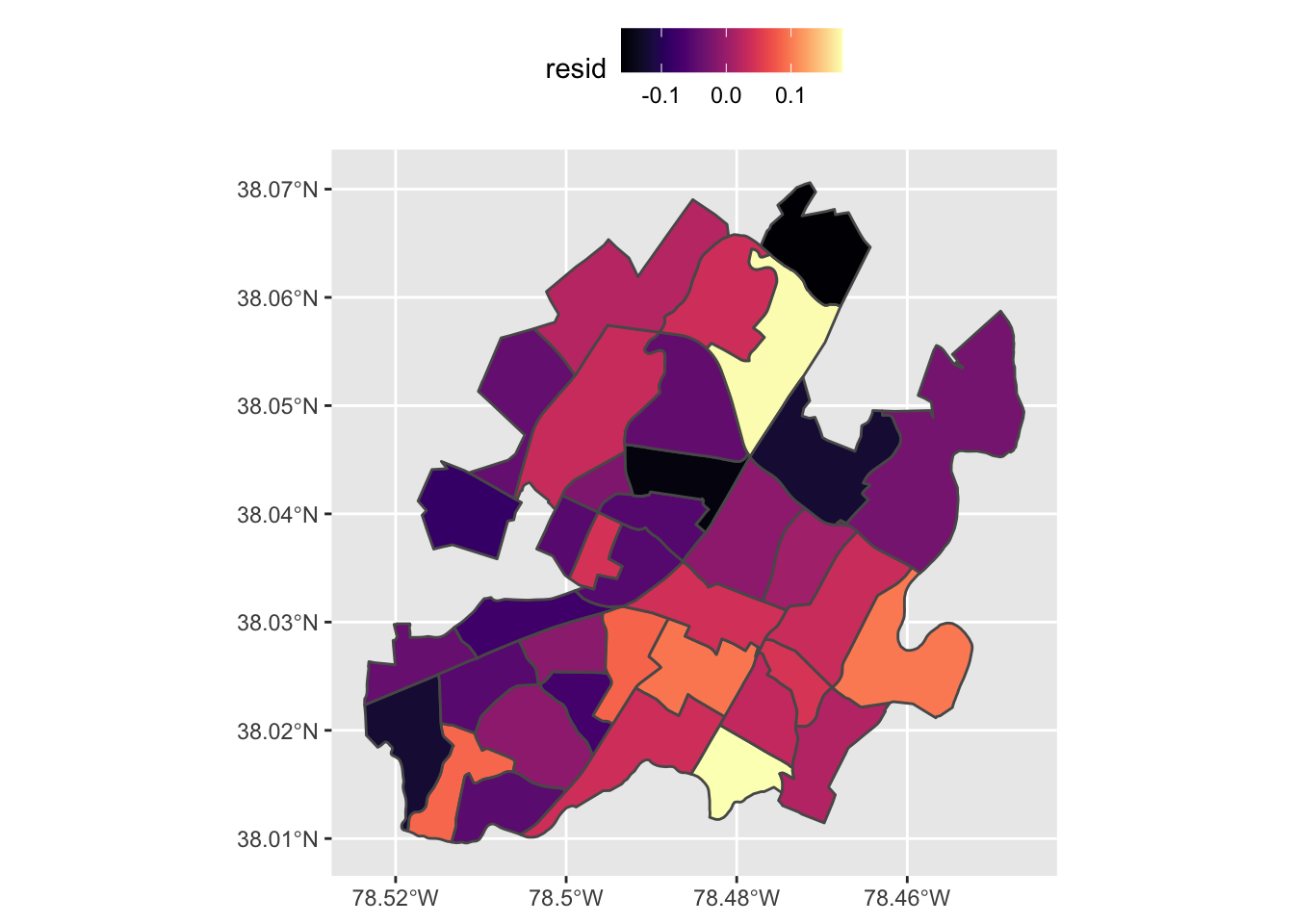

moran.mc(resid(mod), listw = census_wnb, nsim = 99)

## 
##  Monte-Carlo simulation of Moran I
## 
## data:  resid(mod) 
## weights: census_wnb  
## number of simulations + 1: 100 
## 
## statistic = -0.064084, observed rank = 31, p-value = 0.69
## alternative hypothesis: greater

We see a small negative test statistic and we fail to reject the null hypothesis that the residuals are random spatially.

When I first started playing around with the City’s Data Portal back when it launched in August 2017, I wasn’t sure what I would find, but I wanted to focus my #rstats skills on local problems Since I got interested in the crime data, I’ve taken two spatial data courses on Data Camp: Spatial Statistics in R with Barry Rowlingson and Spatial Analysis in R with sf and raster with Zev Ross, which were great and I highly reccommend.

If you have any questions, comments or ideas for future projects, please drop me an email. I’m really looking forward to hosting the Smart Cville Open Data Deep Dive next week, so if you want to learn and play with these tool come out, code and meet some cool civic nerds in the community.